Summary

I train a toy language model to perform two-digit subtraction. I find that the model exhibits grokking (memorization -> generalization) during training, and find that some of the signal in the activations is periodic (like in Neel Nanda’s modular addition paper).

Intro

I’m trying to skill up into AI / Transformer Language Models / Mechanistic Interpretability research. I’m a huge fan of Neel Nanda (and co-authors’) paper on modular addition, so I want to study a language model trained on a task that I bet will learn something similar to what was found in that paper (namely, a trig identity). I’m going to train a simple transformer to perform two-digit subtraction.

Model Details

I’m going to be using the TransformerLens package to set up and analyze the transformer. I’ll train a transformer to perform two-digit subtraction. The input to the model is of the form “” where integers . The numbers and are encoded as 103-dimensional one-hot vectors, where the vocabulary contains 0-99, +, -, and =. The model predicts both the sign and the value of the answer, so valid outputs would be e.g., “50-72=-22” and “43-8=+35”.

I’ll study a one-layer transformer with , learned positional embeddings, four attention heads of dimension , and hidden dimensions in the MLP layer, and I will use ReLU as my activation function.

There are only valid two-digit subtraction problems, and I will use 30% of those () to train the model. I use mini-batch stochastic gradient descent with batch size 256 using the AdamW optimizer with maximum learning rate and weight decay parameter . The learning rate linearly increases from to over the first 5% of training epochs and then decreases using a cosine annealing schedule for the rest of the training epochs. (Note to future self — this is achieved using PyTorch’s SequentialLR). I train for 2000 total epochs.

Training Dynamics

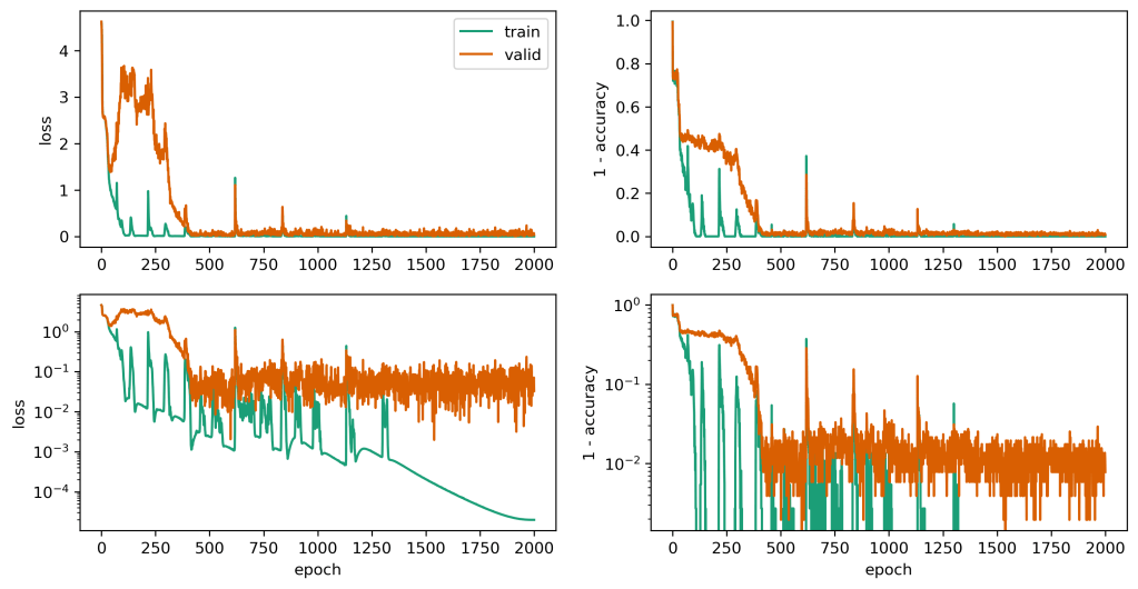
This model exhibits grokking. We see that the loss and accuracy of the train data quickly become small while the validation loss and accuracy remain high (see below). After a few hundred epochs, the validation loss becomes small. Surprisingly, there are a number of ‘spikes’ in the loss curve. I don’t know what’s happening in the model, but I bet it’s finding a bunch of valid solutions and jumping between them (or maybe my learning rate was too high, or maybe I just got unlucky with my batches, or maybe there was too much momentum from AdamW). As I’ll show, the model uses key frequencies to perform its calculation, and these peaks probably represent changes in the dominant frequencies it uses. Note here that I’m calculating the training loss using the full training set (30% of the problem space), whereas I’m only sampling one batch of size 256 to calculate the validation loss / accuracy each epoch.

Matrix Periodicity

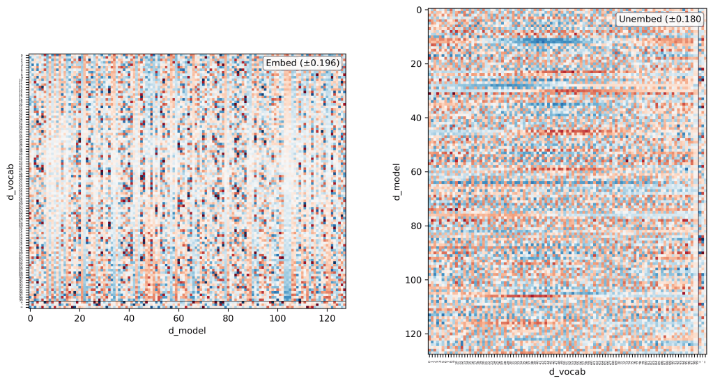
Each dimension of the model exhibits clear periodicity in both the embedding and unembedding matrices. Specifically, this periodicity appears in the d_vocab direction in each dimension of the model. Below is a figure of the embedding and unembedding matrices, where the color shows the weight magnitude, and the colorbar is symmetric around the labeled value in the text box:

If we take a Fourier Transform in the d_vocab direction for each of these matrices, then form the power spectrum, then take the mean power over the model dimension direction, we get the following spectra:

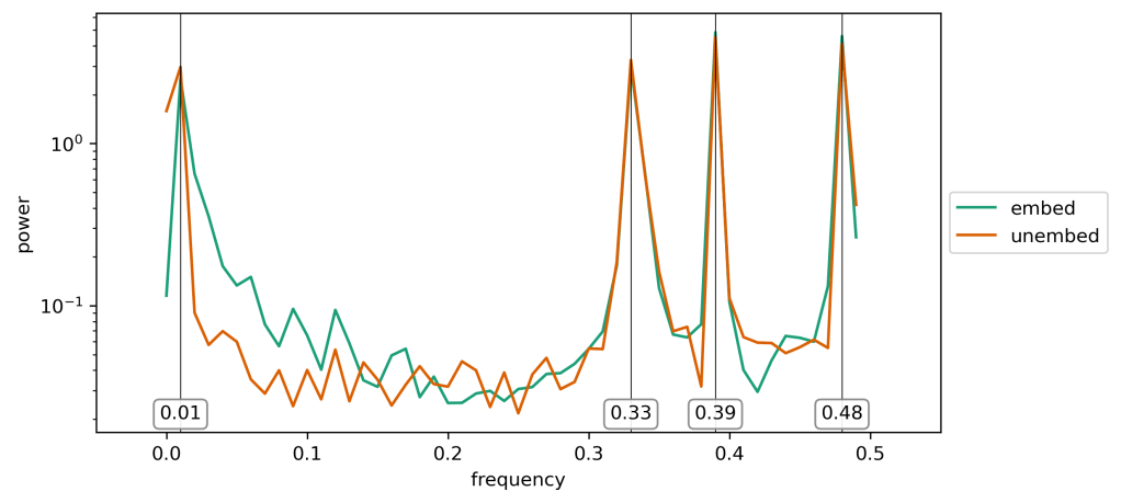
So it looks like the model basically turns our tokens into, primarily, four dominant frequencies which are noted above. Very cool. Although, as we’ll see below, the peak at is a red herring! The bump that extends from that frequency to higher frequencies is very real and important to the model.

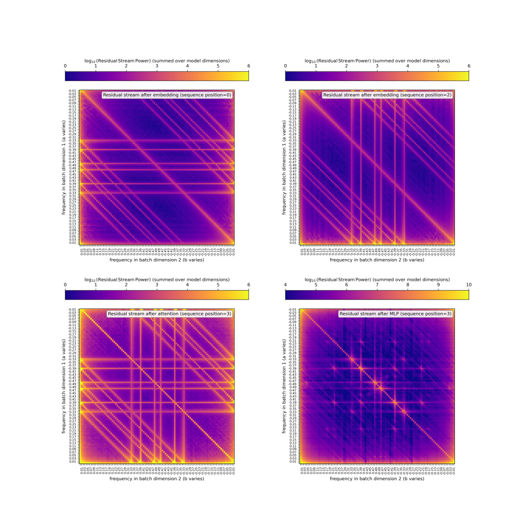
What do the residual stream activations look like?

Fortunately this problem lives in a small universe. There are 100 possible values of and each, and we’ve seen that the vocabulary space (embedding/unembedding) has a high periodicity as a token value changes from [0-99]. So we can shove all of the 2 digit subtraction problems that exist into a batch, split up the samples into two batch dimensions in a [100, 100, …] matrix of problems, run that matrix through the model, then take a 2D Fourier Transform along each of the batch dimension of pretty much any activation or preactivation we’re interested in and look at how our model looks in frequency space. So e.g., if I wanted to look at the residual stream, I would have a matrix of shape [100, 100, n_seq, d_model], and I could transform over the first two dimensions to get the transform, form the power spectrum, then select one the sequence position of interest and sum over all d_model to get a sense of the power spectrum (this is what I do below).

I’m being largely inspired by Chapter 1, part 5 ARENA notebook in my thinking of this problem, and wanted to shout that out before I move ahead. In that notebook, Fourier Transforms are taken with custom functions, but I’m going to be using the NumPy FFT module in this analysis. The FFT module projects onto a basis of complex exponentials (e.g., a series in time would be projected for frequencies onto the functions), so I will have positive and negative frequencies, and my axes will go from low frequency, to high frequency, to negative high frequency, to low frequency — this just means that the low-frequency stuff is at the edges and the high frequency stuff is in the middle.

Below I plot the 2D transformed activations of four different spots within the model’s context. In the upper row, I plot (left) the embeddings in the residual stream at sequence position 0 ( in our problem) and (right) the embeddings in the residual stream at sequence position 2 ( in our problem). In the bottom row I examine sequence position 3 (the ‘=’ sign, and the position responsible for predicting if a + or – comes next); I show the residual stream after the attention operation (left) and after the MLP has operated.

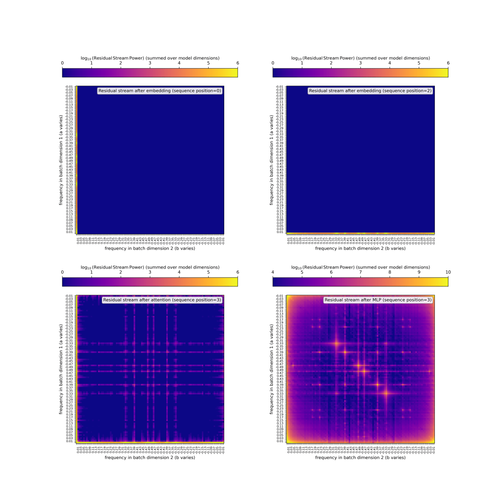
There’s a few features to note:

• The activations of token are simple periodic functions along batch dimension 0 (this makes sense, they vary smoothly from 0 to 100 along that dimension).
• Similarly, the activations of token are simple periodic functions along batch dimension 1 (makes sense for the same reason as above).
• Attention largely seems to be copying the power from each of those positions into position 3. I haven’t verified that it’s doing this, but it’s moving power into the same spots in frequency space, so it’s at least copying-adjacent. (Although, from looking at this in more detail later, it’s certainly doing something more complicated than copying! It would be fun to figure this out.)
• The MLP is spraying power from low frequencies to higher frequencies, and is making things much less sparse!

The last of these things is upsetting and complicated, so I’ll look into that a bit below, but first I want to quickly note that above I’m showing the power spectra for all possible problems. If I instead just look at e.g., the problems with a negative result (edit: I do this by forming a [100, 100] mask of bools which are 1 for a negative result and 0 for a positive result, and I multiply my activations by this mask before transforming — I think this is not necessarily the ‘right’ way to look at just negatives, and this is part of why I get confused below), I get the spectra below:

My interpretation here is largely the same — it’s just interesting to me that including all of the positive and negative problems in my batch manages to cancel out these extra features in the power spectra. I would naively think “both have equal and opposite power at the same frequencies, so they should add their power together and reinforce the features you see!” But — that’s not what’s happening. Maybe I’m just unfamiliar with how 2D FTs work, or maybe I’m thinking about this wrong. Interested in feedback / thoughts here.

In what way are the activations not sparse in frequency space?

So we see above that the activations are not as sparse as hoped in frequency space. This can be seen in a couple of ways, namely: power occupies many frequencies in the first row / column of e.g., the embeddings and post-attention, and also power occupies…a lot of the plot after the MLP acts.

It turns out that power is enveloped by a really simple power law (for the frequency). The model then learns a few key frequencies (as we saw above) on top of that. I think the power law relates to the part of the model that predicts the token, and the key frequencies are used to predict the subtraction value in ). Here’s a few plots slicing out the leftmost or bottommost row of some of the above power spectra plots and showing that is a pretty good fit to the frequency spectrum:

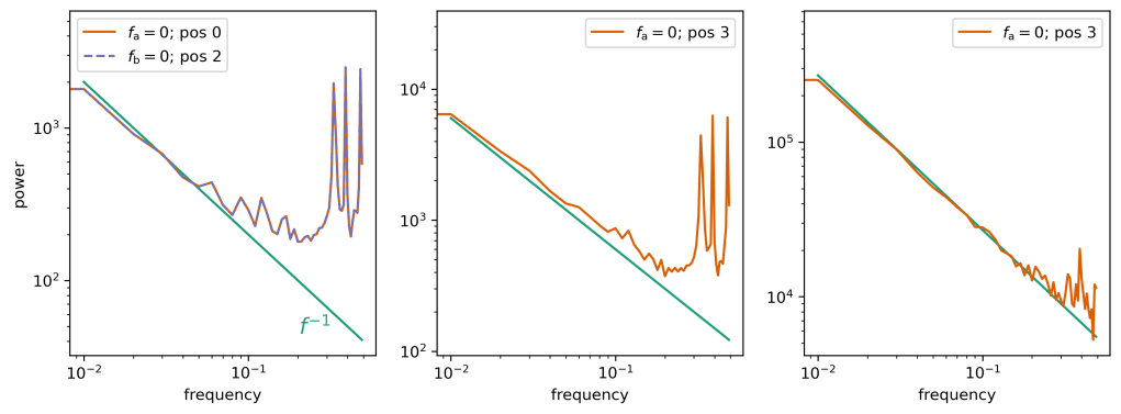
One of the reasons that I think that the “key frequencies” aren’t used in predicting the token is because they’re pretty much obliterated at this sequence position in the MLP. Also — if you take the 2D Fourier Transform of the post-MLP residual stream, ablate all high frequencies (e.g., all frequencies above ), then transform back, unembed, and calculate the logits, loss, and accuracy, then the loss on calculating the $\pm$ token only increases from 0.068 to 0.08 and the accuracy only decreases from 98.55% to 98.21% despite all of the high key frequencies being ablated.

Wrap up & Code Availability

So my choice to split the +/- out from the last value resulted in what looks like a really different algorithm being learned by the model for the prediction of one of the two output tokens! Here I’ve got an initial handle on what the landscape of the activations look like, and in my next post I’ll try to nail down exactly what the function is that the model is using to calculate the token.

The code I used to train the model can be found in this colab notebook, and the code I used to create the plots can be found in this Github repo, which I’ll update as I continue along this project!

Acknowledgments

Big thanks to Adam Jermyn for helping me find my footing into AI safety work and for providing me with mentorship and guidance, and also for providing feedback on an early version of this blog. Thanks also to Neel Nanda for recommending that I keep a record of small projects (like this one!) in blog form as I skill up.