Summary
I continue studying a toy 1-layer transformer language model trained to do two-digit addition of the form 


Intro
In previous posts, I described training a two-digit subtraction transformer and studied how that transformer predicts the sign of the output. In this post, I look at how the model’s weights have been trained to determine the difference between two-digit integers, and the emergent behavior of model activations.
Roadmap
Unlike in my previous post, where I worked back-to-front through the model, this time I’m going to take the opposite approach, starting at the input and understanding how it transforms into the output. I will break down in order:
- The attention patterns, and which tokens the model attends to to predict the output.
- The neuron activations, including:
- How the attention head weights set the pre-activations.
- The emergent patterns in the pre-activations.
- The emergent patterns in the activations.
- The mapping between neurons and logits.
- The patterns in the logits.
Attention Patterns
Here’s a visualization of the attention patterns for four examples (two positive, two negative, using the same numerical values for a and b but swapping them):

I’ve greyed out all of the unimportant rows so we can focus on the second to last row, which corresponds to the row where the transformer predicts the number c. There’s a few things to notice here:
- When the result is positive, H0 attends to token b and H3 attends to token a.
- When the result is negative, H0 attends to token a and H3 attends to token b.
- H1 and H2 roughly attend roughly evenly to all tokens in the context.
So H3 always attends to whichever of a and b has a larger magnitude, and H0 always attends to whichever has the smaller magnitude. H1 and H2 don’t seem to be doing anything too important.
In math, the above intuition can be written as the attention paid to token a by each head:

and the attention paid to token b by each head:

where 

Neuron Pre-Activations and Activations
The function(s) implemented by attention heads
The matrix 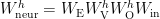


Here are the four types of patterns that I see in the head contributions to the neuron activations:

So neuron 17 basically contributes linearly, and many other neurons have different types of oscillations. If we fit a line to each head’s contribution to each neuron, subtract that, and then transform these signals into frequency space, we can form the following power spectra:
Here I’ve placed vertical lines at the three key frequencies (0.33, 0.39, 0.48) which I saw in my initial post on this topic. We see:
- The small oscillations on top of the linear trend in neuron 17 have a few peaks in the frequency spectrum associated with these key frequencies, but they’re weak.
- Neuron 5 has strong peaks associated with each of these key frequencies, but the peak at
is by far the strongest. Second, this dominant peak is not completely sharp. It has a strong central value as well as fairly strong “feet” values immediately to the side of the central value. This will be important in a sec.
- Neuron 76 is a mess. And there are a decent number of neurons like this. There’s a strong peak but also a spread of power away from that frequency, falling off something like
.
- Neuron 125 exhibits strong beats in the token signal and this corresponds to a gradual increase of power towards the peak at f = 0.48. This again is kind of a bit of a mess.
So what we’re seeing is that these peaks can be described mostly in terms of a strong central peak and corresponding strong peaks in the frequency bins right next to that central peak. This is very reminiscent of the apodization of peaks we see in signal processes when we use windowing techniques — power from a sharp central peak gets spread out a bit into adjacent bins.
I’m not entirely sure what the right function is to generally fit these functions, but this seems like as good a guess as any:
![\tilde{n}_{i,h}(t) = \underbrace{\left(m t + c\right)}_{\rm linear} + \sum_{i}^{0.33, 0.39, 0.48} \left[a_i \underbrace{\cos(2\pi f_i t + \phi_i)}_{\text{central peak}} + \underbrace{b_i\cos(2 \pi f_i t + \theta_{0,i})\cos\left(\frac{2\pi}{d_{\rm vocab}'} t + \theta_{1,i}\right)}_{\text{"feet" of central peak}}\right]](https://s0.wp.com/latex.php?latex=%5Ctilde%7Bn%7D_%7Bi%2Ch%7D%28t%29+%3D+%5Cunderbrace%7B%5Cleft%28m+t+%2B+c%5Cright%29%7D_%7B%5Crm+linear%7D+%2B+%5Csum_%7Bi%7D%5E%7B0.33%2C+0.39%2C+0.48%7D+%5Cleft%5Ba_i+%5Cunderbrace%7B%5Ccos%282%5Cpi+f_i+t+%2B+%5Cphi_i%29%7D_%7B%5Ctext%7Bcentral+peak%7D%7D+%2B+%5Cunderbrace%7Bb_i%5Ccos%282+%5Cpi+f_i+t+%2B+%5Ctheta_%7B0%2Ci%7D%29%5Ccos%5Cleft%28%5Cfrac%7B2%5Cpi%7D%7Bd_%7B%5Crm+vocab%7D%27%7D+t+%2B+%5Ctheta_%7B1%2Ci%7D%5Cright%29%7D_%7B%5Ctext%7B%22feet%22+of+central+peak%7D%7D%5Cright%5D&bg=ffffff&fg=000&s=0&c=20201002)
where 
I use scipy’s curve_fit to fit functions of the form 


I now replace the neuron preactivations with these fits (using the attention patterns I discovered in the previous section). I also keep the biases that end up being important: I find that the value bias from the attention heads and the embedding and positional embeddings (so the original residual stream that goes into the attention operation at context position 4) are important in setting the neuron preactivations.
When I make this approximation, loss increases on all
The resulting neuron pre-activations
In the previous section I examined how the model weights set the neuron pre-activations, but now I’m just going to look at the pre-activations and see if I can understand a simpler algorithm for describing them.
The previous section left me convinced that there would perhaps be four different classes of neurons. But, after a lot of struggling, it turns out there are only two, and both can be described using a simple fit:

where there is a linear portion (slope 


The thing is — this fit is only implemented by the model in the region where 


![a \in [50, 99]](https://s0.wp.com/latex.php?latex=a+%5Cin+%5B50%2C+99%5D&bg=ffffff&fg=000&s=0&c=20201002)
![b \in [0, 49]](https://s0.wp.com/latex.php?latex=b+%5Cin+%5B0%2C+49%5D&bg=ffffff&fg=000&s=0&c=20201002)
To see how this works, here are some sample neuron pre-activations (top row) and these fits (bottom row):

These fits look really pretty good! If I go into the model and replace all of the neuron pre-activations with best-fits to 
The Neuron Activations
The ReLU() is our one nonlinearity in the problem. It spreads power from the nice fit I described above outwards. Specifically, I find (similar to Neel’s grokking work) that
![\text{ReLU}[A_1\cos(\omega_i a + \phi_1) + A_2\cos(\omega_i b + \phi_2)] \approx \frac{1}{2}\left[A_1\cos(\omega_i a + \phi_1) + A_2\cos(\omega_i b + \phi_2)\right] + A_3\cos(\omega_i a + \phi_1)\cos(\omega_i b + \phi_2).](https://s0.wp.com/latex.php?latex=%5Ctext%7BReLU%7D%5BA_1%5Ccos%28%5Comega_i+a+%2B+%5Cphi_1%29+%2B+A_2%5Ccos%28%5Comega_i+b+%2B+%5Cphi_2%29%5D+%5Capprox+%5Cfrac%7B1%7D%7B2%7D%5Cleft%5BA_1%5Ccos%28%5Comega_i+a+%2B+%5Cphi_1%29+%2B+A_2%5Ccos%28%5Comega_i+b+%2B+%5Cphi_2%29%5Cright%5D+%2B+A_3%5Ccos%28%5Comega_i+a+%2B+%5Cphi_1%29%5Ccos%28%5Comega_i+b+%2B+%5Cphi_2%29.&bg=ffffff&fg=000&s=0&c=20201002)
So power gets projected outward from the single-axis terms into cross-axis terms.
If I subtract the linear term from the neuron activation fits 
Perversely, if I instead modify that prior guess so that the magnitude of the cross-frequency term is boosted, performance is much better! More concretely, I take the same procedure above, but after fitting I boost 

I’m not completely satisfied with my explanation here, but I also want to wrap up looking at this toy problem before I take vacation tonight from Christmas through New Year’s, so let’s move along!
Neuron-to-logit operation
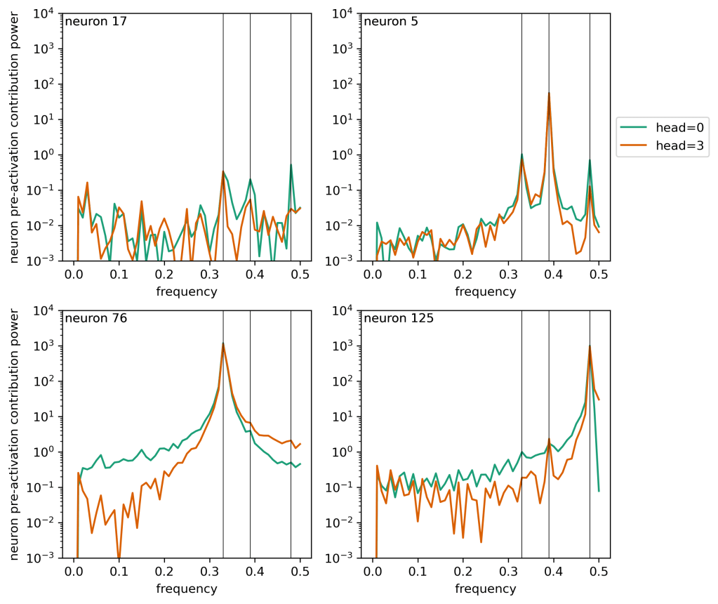
If the neuron activations 

If I Fourier Transform 

There are a number of neurons like neuron 10 on the left. This neuron in particular suppresses low-value logits and boosts high-value logits when a and b are both large (this can be read off from a combination of the top and middle row plots). Neuron 17, in the second row, boosts the logit values of small number tokens and large number tokens (the latter of which seems like an error in what the model learns?) but suppresses intermediate valued tokens when a and b are similar in magnitude and are both small. In both cases, the dominant frequency in the
The right two plots show a different story. Neurons 75 and 125 are oscillatory, and they affects the logits in an oscillatory fashion. The oscillations of the
So if I was right in the previous section and the oscillatory neurons have terms like 

for some amplitude 


where 
In the end, the logits themselves are constructed from a sum over the neurons 
The Logits
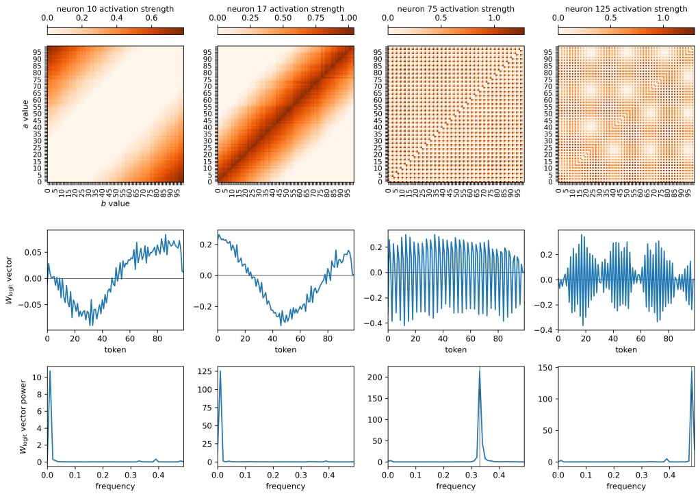
In the end, we get logits that look like this (plotted here are logit maps for 0, 25, 50, an 75):
One thing that pops out to me is that the patterns are no longer oscillatory in two dimensions — they seem to be oscillatory solely in terms of the value of (a – b). This suggests that the model sets the values of 


This also makes intuitive sense: along the diagonals in the (a, b) plane I’ve plotted above, the result of subtraction is always the same! If you increase a by one and also increase b by one, the difference between the two remains the same. So it makes sense that the model would learn a solution that varies and oscillates in the (a-b) direction but which is perfectly constant along the direction perpendicular to that. Neat!
Wrap up
I feel ~85% confident that I’ve figured out the algorithm that this model is using to do subtraction. There are a few spots (particularly towards the end, after the activation function) where things got a bit rushed and hand-wavey, and if I had infinite time to spend on this model then I would solidify and polish some of the concepts there. But I don’t!
I’m going to call it quits on this model and move on to something else perhaps a bit more interesting in my next post, but if anyone has any ideas of holes in my analysis or thoughts about things the model might be doing that I’m not examining, I’d be happy to discuss!
Code
The code I used to train the model can be found in this colab notebook, and the notebook used for this investigation can be found on Github.
Acknowledgments
Thanks again to Adam Jermyn for his mentorship and advice, and thanks to Philip Quirke and Eoin Farrell for our regular meetings. Thanks also to Alex Atanasov and Xianjun Yang for taking the time to meet with me and chat ML/AI this week!

Leave a comment